An interface for exploring space-time
manifolds of time-lapse image sequences
Aseem "Poppa" Agarwala
Ben "Disco Stu" Stewart
Jonathan "Fu Manchu" Ko
Of the many challenges in the creation of time-lapse mosaics it is the
last step, the choice of compositing scheme, that is arguably the least
constrained. After the images have been aligned, blended and
adjusted for other effects such as lighting and exposure, the task of
creating a composite image still remains. Given a sequence of
images depicting a time-lapse sequence we wish to visualize, how do we
create a single composite? The decisions inherent in this step are
highly dependent upon the specific sequence and should be left to the
user. We thus present a novel interface that will allow a user
to create a composite image from a time-lapse sequence.
1. Problem Statement
Let  be a sequence of
  images
  of dimension
  . The problem is to
create a composite image
. The problem is to
create a composite image  , also of dimension , where each pixel
  is chosen from the set
  . Therefore each
pixel of
is represented by a variable
. Therefore each
pixel of
is represented by a variable  ,
ranging from 1 to , that indicates the image
,
ranging from 1 to , that indicates the image  from which the pixel is
chosen. When is not an integer, the
pixel value can be calculated using linear interpolation. The
resultant image can be considered a manifold in
the space-time of a time-lapse image sequence.
from which the pixel is
chosen. When is not an integer, the
pixel value can be calculated using linear interpolation. The
resultant image can be considered a manifold in
the space-time of a time-lapse image sequence.
2. Approach
We thus describe an interface to specifying the values of for the composite image . Clearly, the manual
specification of each of these values is too labor intensive.
Instead, we allow the user to specify a small number of values, and then use
scattered data interpolation techniques to create smoothly varying
values of each across that satisfy the manually specified values.
Of course, specifying an actual value for
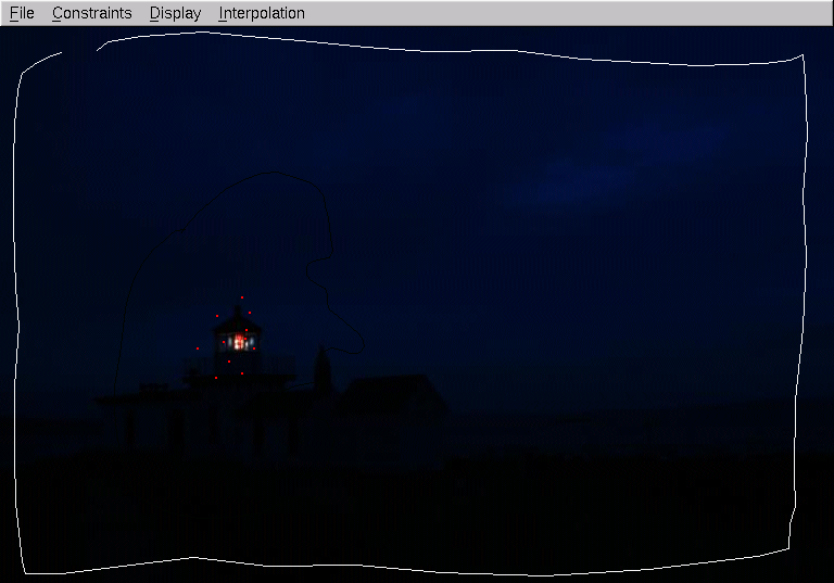
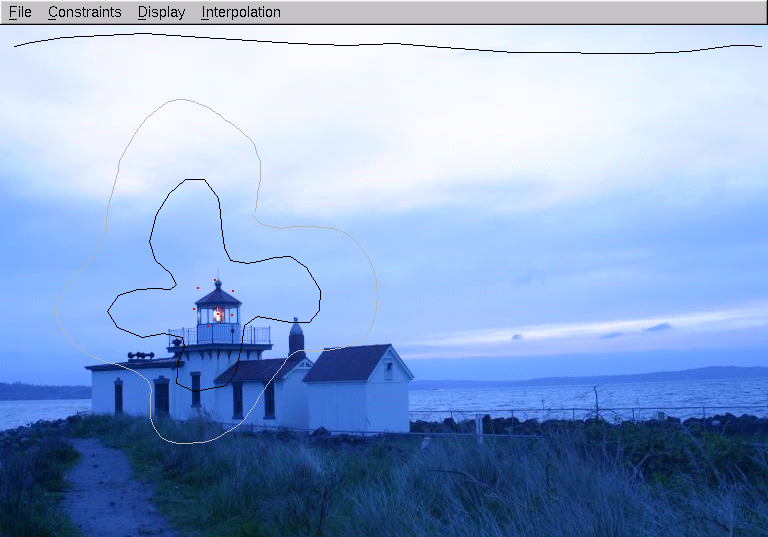
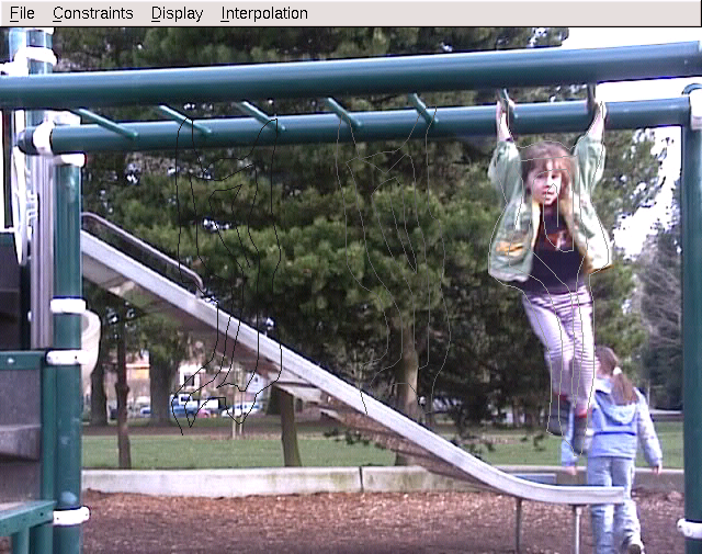
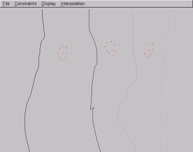
is non-intuitive. Instead, the user draws primitives directly on
the image sequence using a GUI interface; in a sense, the user is
"drawing time." The user can draw points, lines, and regions.
For each pixel covered by a drawn primitive, a value of is specified; the
determination of this value depends on the type of primitive. We
require that drawn primitives do not intersect, to avoid conflicting
assignments of .
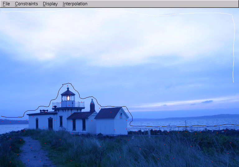
2.1. Points
For this type of drawn primitive, the user scrolls to the appropriate
image i in
the image sequence. The user clicks points directly on this image;
by doing so at location (x,y), he is
specifying that =i. In
this way, the user can ensure that the composite contains the
appearance of the pixel the user is clicking; and since the
interpolation is smooth, the region around the pixel will also likely
look similar to the image i that the user
is seeing in the interface.
2.2. Constant time curves
To create a constant time curve, the user scrolls to the appropriate
image i in
the image sequence. The user can then draw a curve directly on the
image; for all points (x,y) on the
curve, the value is set to i. This
accomplished by sampling points along the curve at a frequency of two,
in units of pixel length.
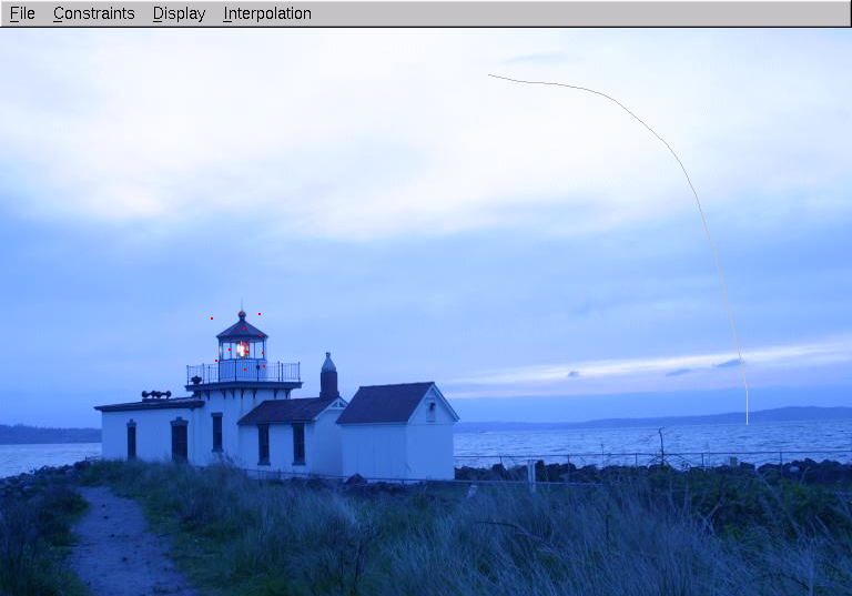
2.3. Varying time curves
This type of curve does not depend on the image that the user is
currently displaying in the GUI. Instead, a curve  is defined parametrically by
  such that
  ,
and
,
and  . For each point
  on a curve such that we set
  . The user can
also alter the time values at the ends of the curve; the default is 1 and n.
. The user can
also alter the time values at the ends of the curve; the default is 1 and n.
Though this type of primitive motivated our approach to this problem as
a whole, we eventually found it to be less useful than planned.
This is because it is difficult for a human to map from such a
curve to the type of effect that will be achieved in the final
composite; this harms the benefits of direct manipulation.
2.4. Painted Regions
The user can also use a paint brush to paint an entire region of an
image i into
the final composite. This type of primitive can be implemented by
sampling the painted region, and defining a point primitive for each
sample.
3. Scattered data interpolation
Once the constraining values of
are defined, the task remains of interpolating these values across
the grid that the
composite spans. We use thin-plate
spline interpolation. This is a physically based 2D interpolation
scheme for arbitrarily spaced, tabulated data. The physical
metaphor is that of a rubber sheet with pins constraining the sheet to
be at a height for each (x,y) where
constraining values are defined. Note that there is no gravity in
this metaphor. The rubber sheet thus smoothly interpolates the
constraining values. It is calculated by minimizing the
bending energy of the sheet. A more complete derivation of
thin-plate splines is out of the scope of this document, but can easily
be found in the literature.
4. Extensions
Along with building and experimenting with this interface, we tried
several extensions.
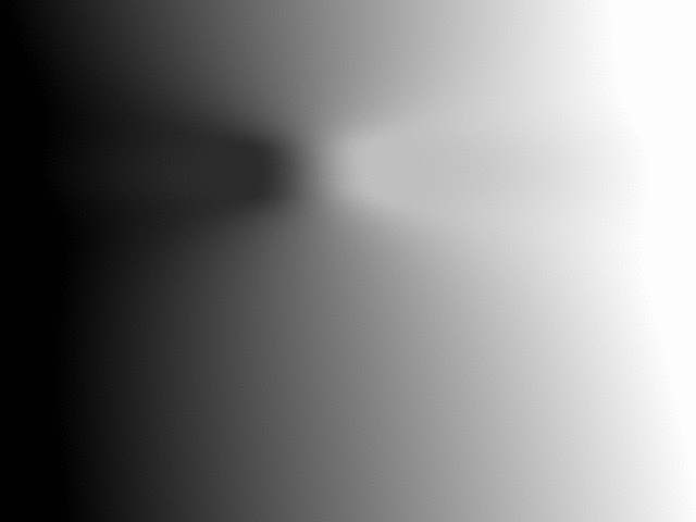
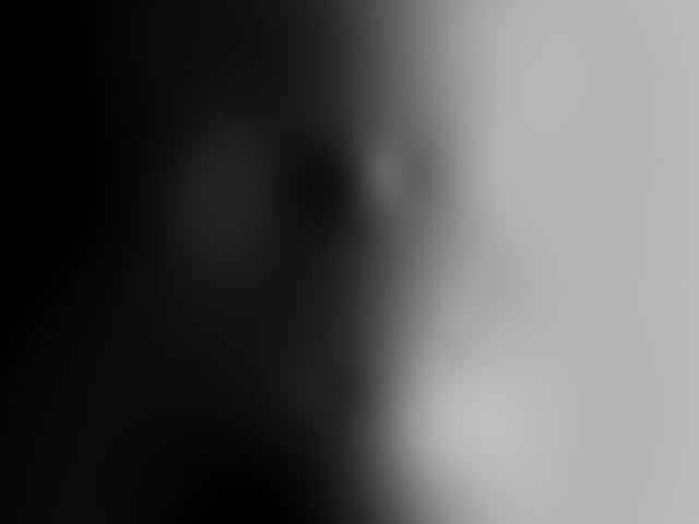
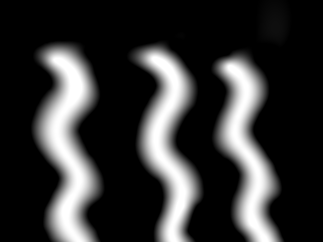
4.1. Images as height fields
One possibility is to use a grayscale image as a height field, to
define the values of . For this process, we create a grayscale image
of size . The grayscale values of this image are
normalized to vary between 1
and n.
We then simply set to this normalized value at each pixel. For a
good result, this grayscale image should be very smooth; thus a
Gaussian blur is usually applied. Also, a time-lapse
sequence that is fairly uniform results in a better appearance;
otherwise, the visual interference of elements of the greyscale image
and elements of the time-lapse sequence can give unintelligible results.
4.2. Animated manifolds
Once we are able to use grayscale images to create composites, we can
also use animated greyscale image sequences.
5. Results
Link to the original Sunset sequence.
Link to the original Candle sequence.
Link to the original Flower sequence.
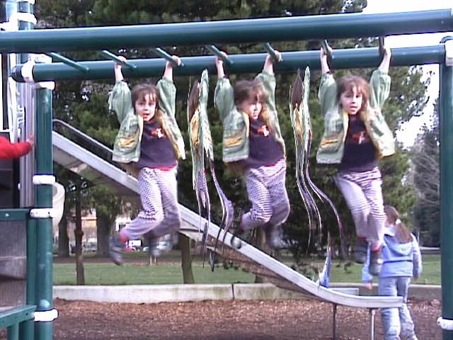
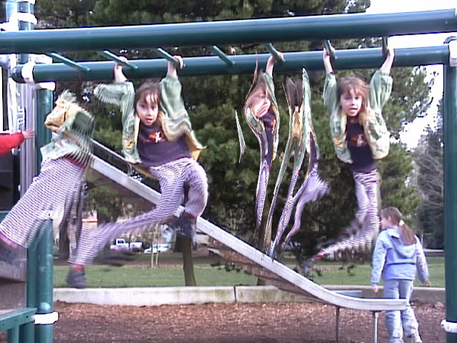
Link to the original Monkeybar sequence. (Removed at request of
original photographer)
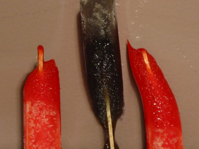
Link to the original Popsicles sequence.
Link to the original Ice sequence.


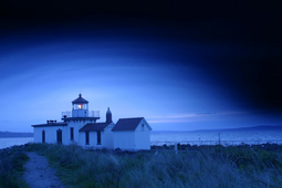
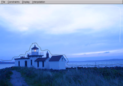
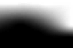

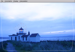

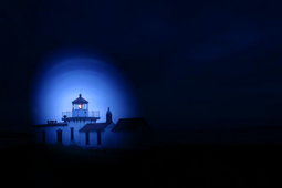
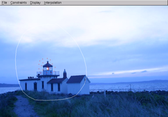
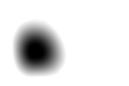
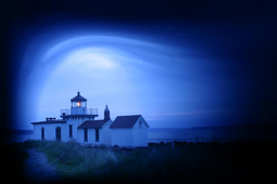
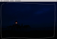
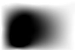
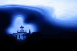
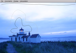


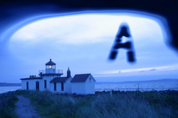


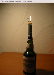

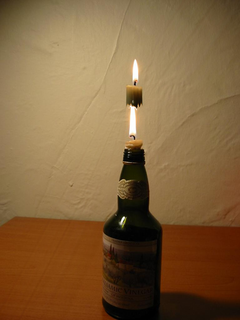
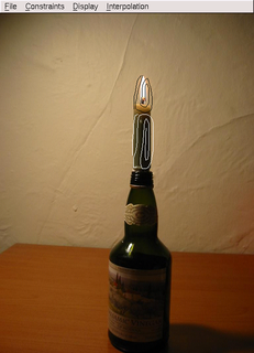


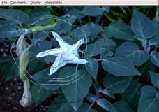


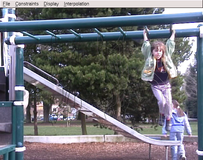
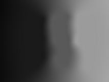
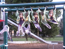
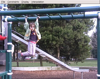

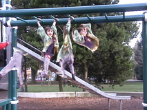
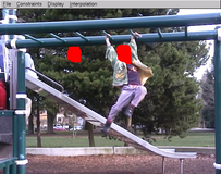
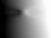
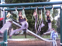
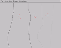
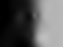

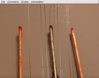
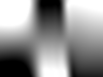
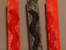
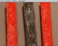

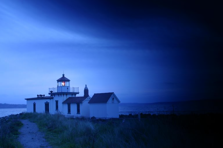
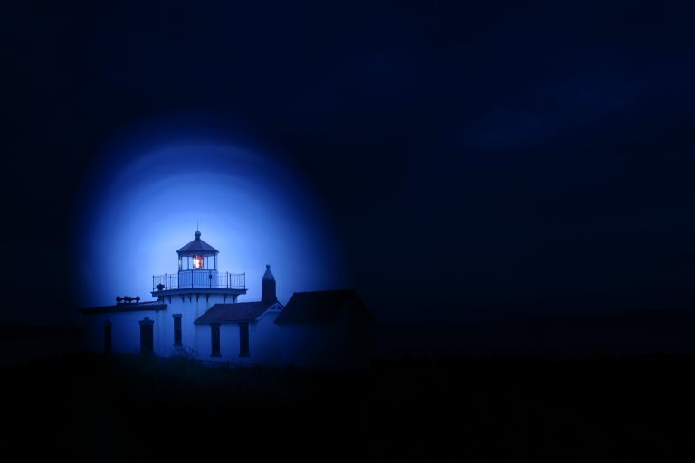
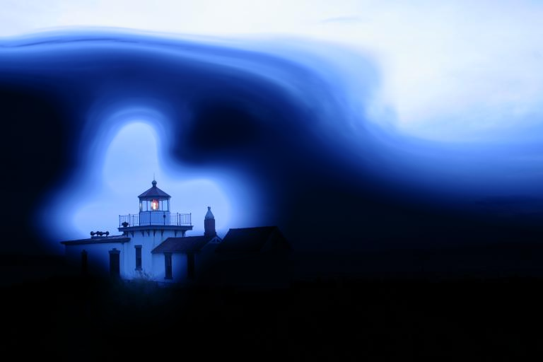
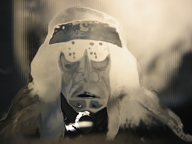
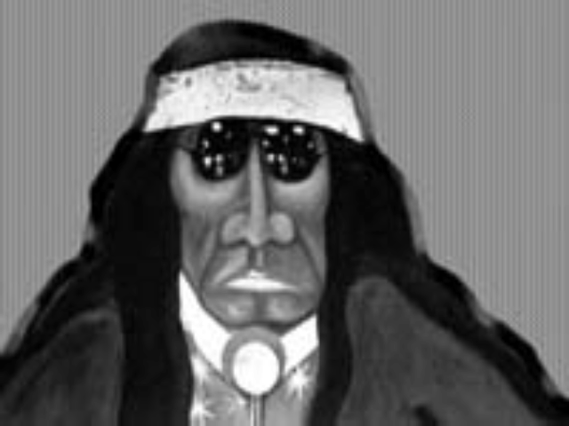
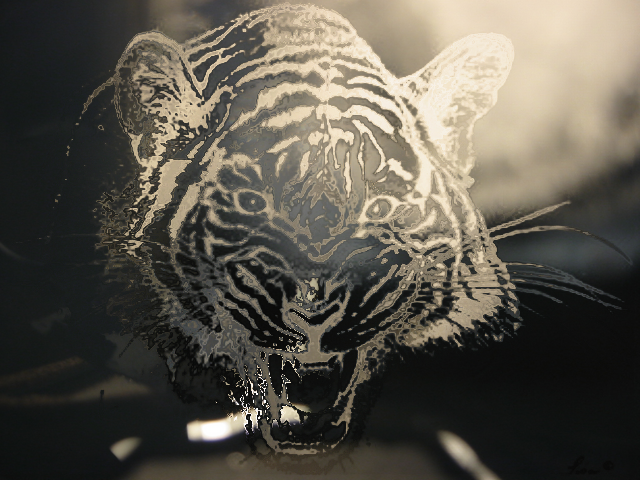
Figure 1: These images were created using the line and point constraints method.


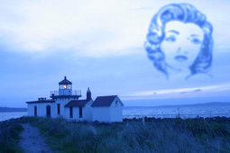


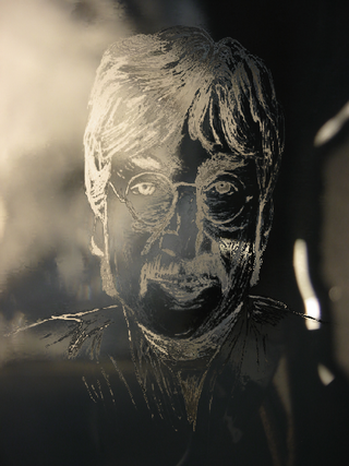
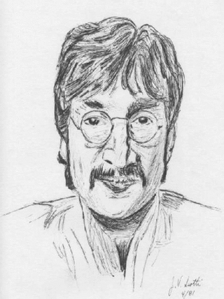
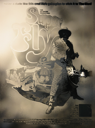

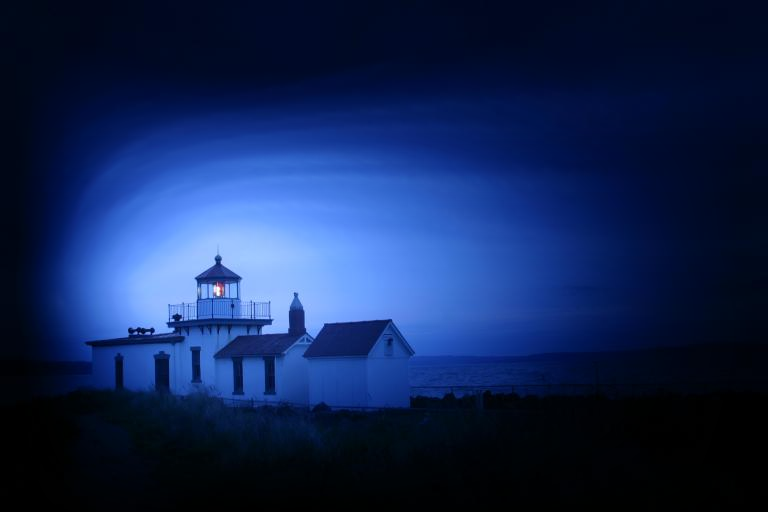
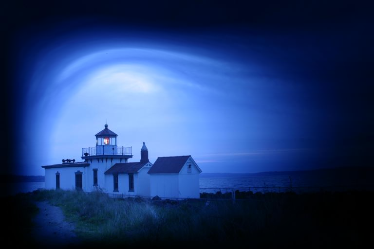
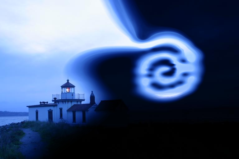
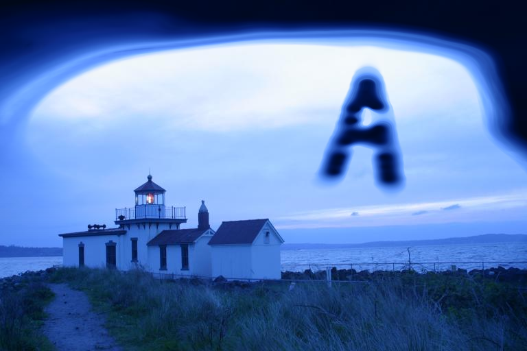
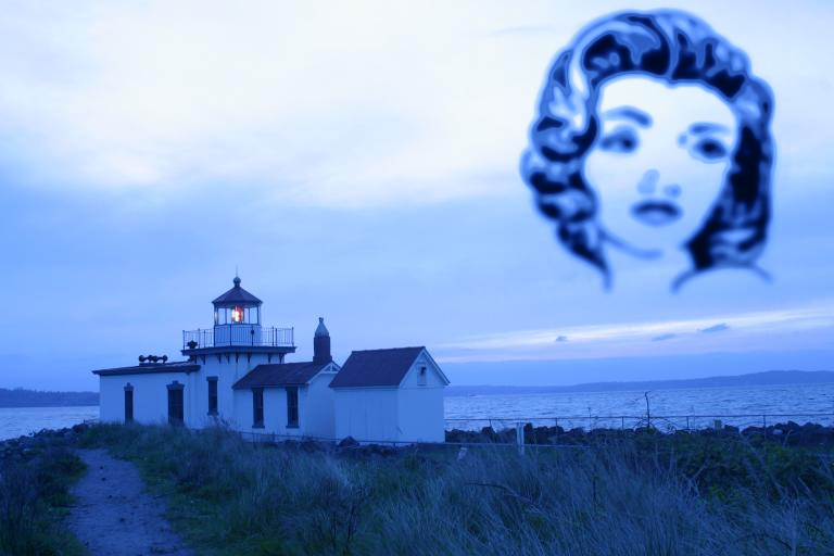
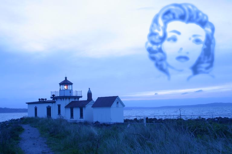
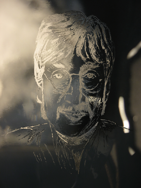
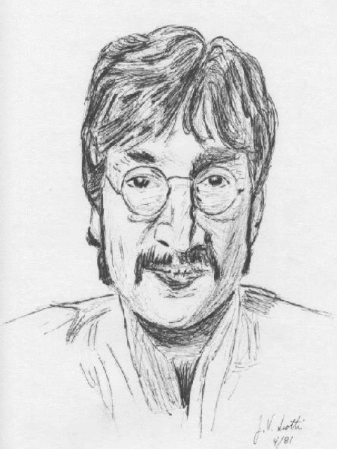
Figure 2: These images were created using the height field method.
Marilyn Ghost animation, height field animation used
Popsicle animation, height field animation used
Figure 3: These animations were created using animated height fields.
6. Future work and conclusion
We have found the interface and methodology presented here very useful
for creating composite images of time-lapse sequences. It was
very entertaining to experiment with the possibilities, and we quickly
learned the mapping between our drawn, constraint primitives and the
resulting composite. This was more true for the first two
primitives; points and constant time curves. These became the
most common tools for us. The time varying curves were less intuitive than originaly thought. Perhaps a mechanism for warping the manifold in 3D would prove more useful. The height field image paradigm produced novel images with ease, but the input sequences used prevented the output images from truly being compelling.
One observation we discovered is that this approach works much better
for time-lapse sequences than for regular video. Regular video
contains much more discontinuous and large motion; this can be
difficult to wrestle into a pleasing composite.
This leads to possibility of higher-level operators for specifying the
pixels used in creating a composite. Perhaps the user could
specify in a more abstract sense what he/she wishes from the composite.
This could be expressed in terms of smoothness and preservation
of edges. Also, the user could delineate objects, perhaps using
intelligent scissors, in certain frames that the composite should
display in as undistorted a way as possible. Then, an
optimization procedure could be run to best satisfy the user
constraints.
Finally, such an optimization procedure could also use constraints from
a target image. The manifold could be chosen so that the
composite resembles the target image as best as possible.